Factorization of polynomials
In mathematics and computer algebra, polynomial factorization refers to factoring a polynomial into irreducible polynomials over a given field.
Contents |
Formulation of the question
Other factorizations, such as square-free factorization exist, but the irreducible factorization, the most common, is the subject of this article.
Factorization depends strongly on the choice of field. For example, the fundamental theorem of algebra, which states that all polynomials with complex coefficients have complex roots, implies that a polynomial with integer coefficients can be completely reduced to linear factors over the complex field C.
On the other hand, such a polynomial may only be reducible to linear and quadratic factors over the real field R. Over the rational number field Q, it is possible that no factorization at all may be possible. From a more practical vantage point, the fundamental theorem is only an existence proof, and offers little insight into the common problem of actually finding the roots of a given polynomial.
Factoring over the integers and rationals
It can be shown that factoring over Q (the rational numbers) can be reduced to factoring over Z (the integers). This is a specific example of a more general case — factoring over a field of fractions can be reduced to factoring over the corresponding integral domain. This algebraic point goes by the name of Gauss's lemma.
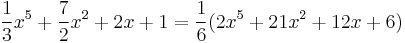
The classic proof, due to Gauss, first factors a polynomial into its content, a rational number, and its primitive part, a polynomial whose coefficients are pure integers and share no common divisor among them. Any polynomial with rational coefficients can be factored in this way, using a content composed of the greatest common divisor of the numerators, and the least common multiple of the denominators. This factorization is unique.
For example,

and
since 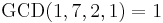 and
and 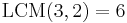 .
.
Now, any polynomial with rational coefficients can be split into a content and a primitive polynomial, and in particular the factors of any factorization (over Q) of such a polynomial can also be so split. Since the content and the primitive polynomials are unique, and since the product of primitive polynomials is itself primitive, the primitive part of the polynomial must factor into the primitive parts of the factors. In particular, if a polynomial with integer coefficients can be factored at all, it can be factored into integer polynomials. So factoring a polynomial with rational coefficients can be reduced to finding integer factorizations of its primitive part.
Obtaining linear factors
All linear factors with rational coefficients can be found using the rational root test. If the polynomial to be factored is  , then all possible linear factors are of the form
  , where
  is an integer factor of
  and
and  is an integer factor of
  . All possible combinations of integer factors can be tested for validity, and each valid one can be factored out using polynomial long division. If the original polynomial is the product of factors at least which two of which are of degree 2 or higher, this technique will only provide a partial factorization; otherwise the factorization will be complete. Note that in the case of a cubic polynomial, if the cubic is factorable at all the rational root test will give a complete factorization, either into a linear factor and an irreducible quadratic factor, or into three linear factors.
Factorizing quartics
Reducible quartic (fourth degree) polynomials with no linear factors can be factored into quadratics.
Duplicate factors
If two or more factors of a polynomial are identical to each other, a situation resulting in multiple roots, then one can exploit the fact that the duplicated factor will also be a factor of the polynomial's derivative, which itself is a polynomial of one lower degree. The duplicated factor(s) can be found by using the Euclidean algorithm to find the greatest common factor of the original polynomial and its derivative.
Kronecker's method
Since integer polynomials must factor into integer polynomial factors, and evaluating integer polynomials at integer values must produce integers, the integer values of a polynomial can be factored in only a finite number of ways, and produce only a finite number of possible polynomial factors.
For example, consider
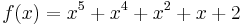 .
.
If this polynomial factors over Z, then at least one of its factors must be of degree two or less. We need three values to uniquely fit a second degree polynomial. We'll use  ,
,  and
and  . Now, 2 can only factor as
- 1×2, 2×1, (−1)×(−2), or (−2)×(−1).
Therefore, if a second degree integer polynomial factor exists, it must take one of the values
- 1, 2, −1, or −2
at  , and likewise at
  . There are eight different ways to factor 6, so there are
- 4×4×8 = 128
possible combinations, of which half can be discarded as the negatives of the other half, corresponding to 64 possible second degree integer polynomials which must be checked. These are the only possible integer polynomial factors of  . Testing them exhaustively reveals that
constructed from  ,
,  and
and  , factors .
(Van der Waerden, Sections 5.4 and 5.6)
LLL algorithm
The LLL algorithm (Lenstra, Lenstra & Lovász 1982), was the first polynomial time algorithm for factoring rational polynomials, and uses the Lenstra–Lenstra–Lovász lattice basis reduction algorithm.
One variation of their algorithm runs as follows: calculate a complex (or p-adic) root α of the polynomial P to high precision, then use the Lenstra–Lenstra–Lovász lattice basis reduction algorithm to find an approximate linear relation between 1, α, α2, α3, ... with integer coefficients, which with luck will be an exact linear relation and a polynomial factor of P.
Factoring over finite fields
See Factorization of polynomial over finite field and irreducibility tests, Berlekamp's algorithm, and Cantor–Zassenhaus algorithm.
Factoring over algebraic extensions
We can factor a polynomial ![p(x) \in K[x]](/2012-wikipedia_en_all_nopic_01_2012/I/b9db1f17d508db907f0a85c531f5be53.png) , where
, where  is a finite field extension of
  . First we eliminate any repeated factors in
  by taking greatest common divisors with its derivative. Next we write
 ![L= K[x]/p(x)](/2012-wikipedia_en_all_nopic_01_2012/I/8e420aa1fc03111fddb1833b2e42e049.png) explicitly as an algebra over . We next pick a random element
explicitly as an algebra over . We next pick a random element  . By the primitive element theorem,
  generates
  over with high probability. If this is the case, we can compute the minimal polynomial,
 ![q(y)\in \mathbb{Q}[y]](/2012-wikipedia_en_all_nopic_01_2012/I/dccb5d4fb4dc6635df6387e7350f79a5.png) of over . Factoring
of over . Factoring
over ![\mathbb{Q}[y]](/2012-wikipedia_en_all_nopic_01_2012/I/01a1ab4f88eb433dc6bda9a9304cef13.png) , we determine that
, we determine that
![L = \mathbb{Q}[\alpha] = \mathbb{Q}[y]/q(y) = \prod_{i=1}^n \mathbb{Q}[y]/q_i(y)](/2012-wikipedia_en_all_nopic_01_2012/I/5ddd6d25d619aa56a99b33b2053a81c4.png)
(notice that is reduced since is), where corresponds to the element  . Note that this is the unique decomposition of as a product fields. Hence this decomposition is the same as
![\prod_{i=1}^m K[x]/p_i(x)](/2012-wikipedia_en_all_nopic_01_2012/I/df8ba0f4e9c9f74d78b8a6fc6df5c18f.png)
where
is the factorization of over ![K[x]](/2012-wikipedia_en_all_nopic_01_2012/I/a77a9131b3530308247cff0e3c92321a.png) . By writing
. By writing  and generators of as a polynomials in , we can determine the embeddings of
  and into the components
 ![\mathbb{Q}[y]/q_i(y)=K[x]/p_i(x)](/2012-wikipedia_en_all_nopic_01_2012/I/89305354777466f463c4425197481ef8.png) . By finding the minimal polynomial of in this ring, we have computed
. By finding the minimal polynomial of in this ring, we have computed  , and thus factored over
See also
Bibliography
- Bernard Beauzamy, Per Enflo, Paul Wang (October 1994). "Quantitative Estimates for Polynomials in One or Several Variables: From Analysis and Number Theory to Symbolic and Massively Parallel Computation". Mathematics Magazine 67 (4): 243–257. doi:10.2307/2690843. JSTOR 2690843. (accessible to readers with undergraduate mathematics)
- Cohen, Henri (1993). A course in computational algebraic number theory. Graduate Texts in Mathematics. 138. Berlin, New York: Springer-Verlag. ISBN 978-3-540-55640-4. MR1228206
- Knuth, Donald E (1997). "4.6.2 Factorization of Polynomials". Seminumerical Algorithms. The Art of Computer Programming. 2 (Third ed.). Reading, Massachusetts: Addison-Wesley. pp. 439–461, 678–691. ISBN 0-201-89684-2.
- Lenstra, A. K.; Lenstra, H. W.; Lovász, László (1982). "Factoring polynomials with rational coefficients". Mathematische Annalen 261 (4): 515–534. doi:10.1007/BF01457454. ISSN 0025-5831. MR682664
- Van der Waerden, Algebra (1970), trans. Blum and Schulenberger, Frederick Ungar.